Technical Appendix
2.2.1.2. For fitting baseline models using the hourly methods, no minimum baseline period length is required.
The baseline period for hourly methods is not set according to a particular time period – one year, for example – but is instead defined as sufficient when the full range of independent variables are observed. This is referred to as “data coverage” in Hourly Methods Documentation. This process is described in greater detail in LBNL’s video on Time-of-Week Temperature models.
2.2.4.1. Temperature data may not be missing for more than six consecutive hours.
The decision to linearly interpolate up to 6 consecutive missing hours of weather data is adapted from Mathieu et al’s Quantifying Changes in Building Electricity Use, with Application to Demand Response (Section 2.2).
2.4.1. Weather station to be used is closest within climate zone that meets CalTrack data sufficiency requirements.
Test 1: Weather station accuracy
Github issue: https://github.com/CalTRACK-2/caltrack/issues/65
Background:
Two weather station mapping methods were considered for CalTRACK 2.0’s data sufficiency requirements. Each proposed weather mapping method is described below:
Method A:
- Determine the candidate weather stations.
- Determine the climate zone standards. The following climate zone standards were considered: a. IECC Climate Zone b. IECC Moisture Regime c. Building America Climate Zones d. CEC California Building Climate Zone Areas
- Establish the site’s climate zone inclusion for each considered climate zone standard.
- Determine each site’s closest candidate weather station.
- Establish the weather station’s climate zone inclusion for each considered climate zone standard.
- Reject the candidate weather station if any of the following are true: a. The candidate station is more than 150 km from the site. b. The candidate weather station’s climate zone does not match the site’s climate zone for all considered climate zone standards. c. The candidate station does not have sufficient data quality when matched with site meter data.
- If criteria in (6) are met, use the candidate weather station. If criteria are not met, move back to step 3 and test the next closest candidate weather station.
- If no stations meet the criteria above, use method B.
Method B:
- Determine the candidate weather station to be considered.
- Determine the (next) closest weather station.
- Reject the candidate station if it does not have sufficient data quality when matched with site meter data
- If no stations meet the criteria above, consider the site unmatched.
Data:
Hourly temperature data from all California weather stations from January 2014 to January 2018. Tested parameters: The weather stations selected based on Method A and Method B were compared against the “ground-truth” weather stations established by a similarity metric.
Testing methodology:
It was problematic to empirically test weather mapping methods on buildings because true temperature values were not available at each site. Although there was no accurate data at the site level, there was accurate data at the location of each weather station. To compare mapping methods, each weather station was considered as a site and weather station selection methods were tested on the weather stations.
The results were compared against a “ground-truth” of weather similarity between weather stations. The “ground-truth” ranking of weather station similarity was determined by a metric that ranked the similarity of a weather station to other weather stations. The similarity metric was constructed with three distance metrics: 1) root mean squared error, 2) kilometers, and 3) cosine distance to the weather station of interest. Weighted equally, these rankings were combined to provide a similarity ranking of all other weather stations for each weather station.
These rankings were the “ground-truth” that compared Methods A and B. After weather stations were selected based on Methods A and B, their accuracy was compared to the “ground-truth” ranking defined by the similarity metric.
Results:
Our results show that Method A produced the best possible weather station 56% of the time and Method B produced the best possible weather station 53% of the time. This indicates that Method A is more accurate than Method B by a small margin.
Test 2: Importance of weather data
Github issue: https://github.com/CalTRACK-2/caltrack/issues/65
Background:
CalTRACK 2.0 methods were designed to be simple and universally applicable. We empirically tested the effect of inaccurate weather data on our model prediction error to determine the importance of weather data accuracy.
Data:
Weather data was collected from two weather stations in each of the 50 states in the United States.
Tested parameters:
Model fit, measured by CVRMSE, was calculated with CalTRACK methods using increasingly inaccurate temperature data.
Testing methodology:
The models from CalTRACK 1.0 were fit with weather data collected from two weather stations in each of the 50 states in the United States. The weather values provided by the geographically and climatically diverse weather stations were largely inaccurate for the buildings observed. This provided an opportunity to analyze the effect of inaccurate temperature data on model fit.
Results:
In the figure below, in-sample prediction error slightly increased as temperature data error increased. These results suggest that small inaccuracies in the weather data have a small effect on model prediction error.
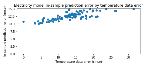
Figure: Model error vs. temperature difference from nearest weather station
Conclusion:
CalTRACK 2.0 will employ Method A as the preferred weather station mapping method, despite the implication that weather station mapping misalignment leads to only a minimal increase in model error. If Method A is impractical or impossible, Method B is a suitable alternative.
3.1.3. Models are fit to baseline data in the 365 days immediately prior to the intervention start date.
Github issue: https://github.com/CalTRACK-2/caltrack/issues/68
Background:
The length of the baseline period in energy savings models may affect energy savings calculations in two ways:
- Periods that are too short may not capture the full range of input conditions, such as weather or occupancy patterns, that are typically experienced by a building.
- Periods that are too long increase the chances of unexpected changes in a building’s energy use. For example, energy efficient equipment unrelated to the intervention is more likely to be added during longer baseline periods. This will affect estimated energy savings.
CalTRACK methods adopt the Uniform Methods Project’s (UMP) minimum baseline period of 365 days (see UMP guidelines in 6.4.1 Analysis Data Preparation). The obvious justification for a 365 day baseline is the value of fitting a model over a wide range of possible temperatures. Hourly methods may require a different baseline length assumption. The UMP does not provide guidance for the maximum length of the baseline period, so empirical testing was conducted to determine the optimal maximum baseline period length.
Data:
Billing period data from approximately 1000 residential buildings in Oregon and daily data from 1000 residential buildings in California.
Tested parameters:
The effect of increasing the length of the baseline period on prediction error.
Testing methodology:
The CalTRACK methods were applied to the full dataset five times using baseline periods of 12, 15, 18, 21, and 24 months for each iteration. The length of the baseline period was the only change between iterations.
Testing was conducted as follows:
- CalTRACK models were fit to each of the candidate baseline periods.
- Total energy consumption predictions for each baseline model we calculated for a 12-month reporting period.
- The CVRMSE and NMBE error metrics were calculated for these predictions.
- This test was conducted separately for daily and monthly data.
Acceptance criteria:
Energy consumption trends and error metrics were compared for different baseline period lengths. The baseline period length that did not inflate out-of-sample errors was recommended as the maximum baseline period length in CalTRACK methods.
Results:
The figure below shows that baseline normalized annual consumption (NAC) increases as the baseline period length increases. This implies that using baseline periods longer than 12 months may unjustifiably inflate estimated savings.
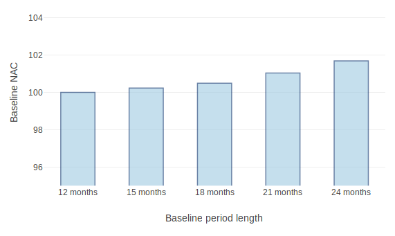
Figure: Effect of baseline period length on normalized annual consumption using daily data
The figure below demonstrates that increasing baseline period length worsened model fit. This may occur because increased baseline periods are more likely to include non-routine events that affect energy use in unpredictable ways.
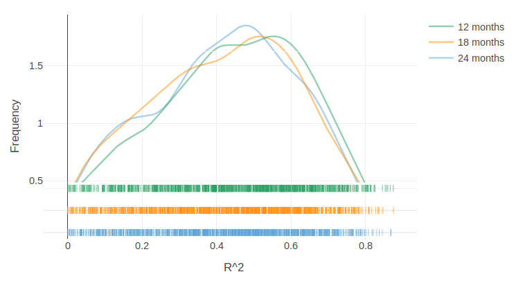
Figure: Effect of baseline period length on model R-squared distribution
Conclusion:
The results from these empirical results indicate that baseline periods longer than 1 year may have increased baseline energy consumption and poorer model fit than the minimum 12-month baseline. We recommend a maximum baseline period length of 12 months for both billing and daily models.
3.1.4.1. Select and qualify balance points for candidate models for each period for each meter.
Github issue: https://github.com/CalTRACK-2/caltrack/issues/69
Background:
CalTRACK 1.0 methods recommends that fixed balance point temperatures are used for degree-day covariates in billing period methods. The UMP recommends fixed balance point temperatures 60 F for heating degree days and 70 F for cooling degree days for billing period methods.
For daily methods, the UMP recommends that variable balance points are used for degree-day covariates.
It is possible that billing period models will have improved model fit with variable balance points instead of the fixed balance points suggested by the UMP.
Data:
Electricity and gas billing data from approximately 1000 residential buildings that had undergone home performance improvements in Oregon.
Tested parameters:
The R-squared of a billing period model using fixed balance points of 60 F for HDD and 70 F for CDD was compared to a model with variable balance point ranges of 40-80 for HDD and 50-90 for CDD.
Testing methodology:
- CalTRACK billing period models were fit to baseline period usage data with fixed balance point temperatures.
- The fitting process was repeated with a grid search for the balance point temperatures with a grid search range of 40-70 F for heating degree days and 60-90 F for cooling degree days. A 3 F search increment was used to determine variable balance point temperatures.
- The error metrics of CVRMSE and NMBE were calculated for each model with fixed and variable balance points.
Acceptance criteria:
Variable balance point temperatures for billing period models were accepted into the CalTRACK 2.0 specification if the variable balance point models did not cause the average model performance to deteriorate. The average model performance did not deteriorate if average model fit improved or a paired t-test of model fit metrics showed no significant difference.
Results:
For the 1077 buildings tested with fixed balance points, 479 were fit using intercept-only models. When the same 1077 buildings were tested with variable balance points, there were 357 intercept-only models. These results indicate that the weather-sensitivity of some buildings was not being modelled with fixed balance point temperatures.
The performance of the remaining weather-sensitive buildings were compared when fit with fixed and variable balance point temperatures. The mean R-squared for fixed balance point models was 0.480, while the mean R-squared for variable balance point models was 0.495. The figure below shows slight improvements in model fit for variable balance point models.
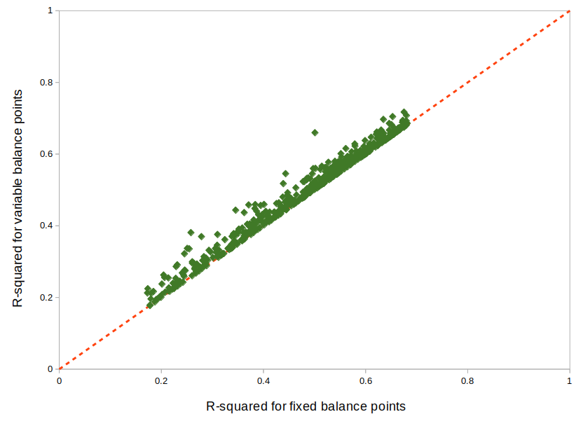
Figure: R-squared for fixed and variable balance points
Conclusion:
Our empirical results indicate that variable balance points generated fewer intercept-only models and had a slightly improved R-squared than fixed balance points in billing period methods. Therefore, we recommend using variable balance points in billing period methods.
3.2.1. A grid search of models is performed using a wide range of candidate balance points.
Github issue: https://github.com/CalTRACK-2/caltrack/issues/72
Test 1: Distribution of selected balance points with different grid search ranges
Background:
Daily and Billing Period methods in CalTRACK 2.0 use variable degree-day regression to model baseline and reporting period energy consumption. In variable degree-day regression, the analyst must establish a search range that contains the optimal balance point temperatures for each degree-day covariate. Excessively large search ranges have high computation requirements. However, overly constrained grid search ranges may lead to suboptimal balance point temperatures and poor model fit. The testing protocol below was used to define the optimal grid search ranges for HDD and CDD covariates.
Data:
Billing period data from approximately 1000 residential buildings in Oregon and daily data from 1000 residential buildings in California.
Tested parameters:
HDD and CDD balance points were calculated with different grid search ranges using Caltrack methods.
Testing methodology:
Caltrack models were fit to the Oregon building usage dataset using 4 balance point search ranges:
- 10-degree range: 55-65 F HDD and 65-75 F CDD
- 20-degree range: 45-65 F HDD and 65-85 F CDD
- 30-degree range: 40-70 F HDD and 60-90 F CDD
- 40-degree range: 40-80 F HDD and 50-90 F CDD
Results:
The bar chart below shows the distribution of best-fit HDD balance points for three of the four tested grid search ranges. These results show that when the grid search is constrained, models tend to select balance points at the end of the grid search range. For the 10-degree grid search range, almost 30% of the buildings have an HDD balance point of exactly 65 F. But when the grid search range is expanded to the 30 F or 40 F ranges, the distribution of best-fit balance points tends towards a Gaussian distribution centered around 63 F. These results indicate that overly constrained grid search ranges may result in suboptimal best-fit balance points and, thereby, suboptimal model fits.
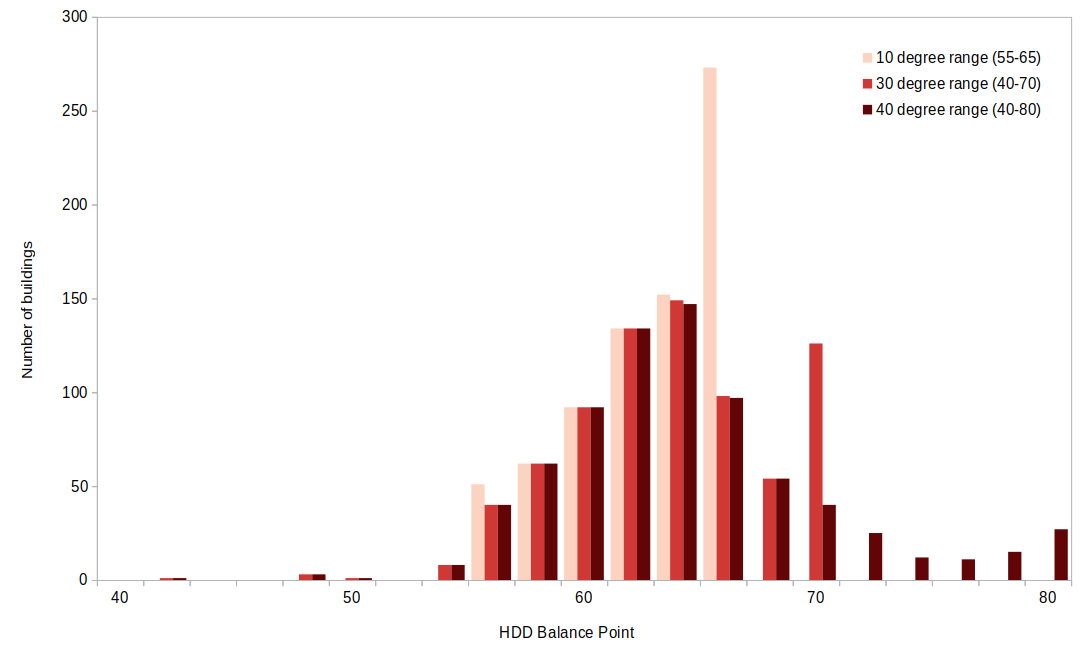
Figure: HDD balance point frequency by grid search range
Test 2: Importance of optimal balance points on estimated savings
Github issue: https://github.com/CalTRACK-2/caltrack/issues/72
Background:
The robustness of estimated savings to different balance point ranges provides more confidence in our estimated energy savings calculations.
Data:
Billing period data from 1000 residential buildings in Oregon and daily data from 1000 residential buildings in California.
Tested parameters:
CalTRACK methods estimated energy savings for all program participants for five different grid search ranges.
Testing methodology:
Baseline models were fit to the full set of program participants five times, varying the search range for the HDD balance point and keeping all other parameters constant. The annualized estimated savings were calculated for each grid search range.
Results:
The box plots below show that estimated energy savings were similar across different grid search ranges. This indicates that estimated savings with CalTRACK methods are robust to varying grid search ranges.
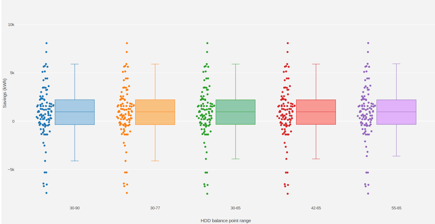
Figure: Estimated savings with different grid search ranges
Conclusion:
Expand balance point search range to 30-90 F for heating balance points and 30-90 F for cooling balance points.
3.2.3. Maximum gap between candidate balance points in the grid search is 3 degrees F or the equivalent in degrees C.
Github issue: https://github.com/CalTRACK-2/caltrack/issues/72
Background:
The grid search algorithm selects balance points by, first, estimating a model with each set of candidate HDD and CDD balance points and, second, choosing the balance points that generate the best-fit model.
The analyst determines the search increments, or “steps”, that the algorithm uses to choose models that are tested for the optimal balance point. Small search increments, such as 1 degree, estimate a model for each degree in the HDD and CDD grid search ranges. This is computationally intensive. Larger search increments have lower computational demands, but could provide less accurate balance points temperatures.
Data:
Billing period data from 1000 residential buildings in Oregon and daily data from 1000 residential buildings in California.
Tested parameters:
The selected balance point temperature with search increments of 1, 2, 3, and 4 degrees.
Testing methodology:
CalTRACK methods were used to estimate models with balance point temperatures selected with search increments of 1, 2, 3, and 4 degrees. The results were compared to determine the optimal search increment.
Results:
The empirical results show that model fit did not change significantly when balance points were off by 1 F. This implies that a search increment of 3 F is acceptable because the optimal balance point temperature can only be 1 F above or below the optimal balance point with a 3 F search increment.
Figure: HDD balance points with different search increments
Conclusion:
CalTRACK’s Billing Period and Daily methods will use a 3 F search increment in the grid search algorithm.
3.3.1.2. Independent variables
Test 1: Calendar effects and error structure
Github issue: https://github.com/CalTRACK-2/caltrack/issues/57
Background:
CalTRACK models are specified with only HDD and CDD covariates. However, there are a priori reasons to expect that energy consumption could be correlated with calendar effects, such as day-of-week, day-of-month, month-of-year, or holidays. If calendar effects are significantly correlated with energy consumption and excluded from the model, it may cause less accurate energy savings estimates with poorer model fit. .
Calendar effects can be added to the model as categorical variables for day-of-week, day-of-month, month-of-year, or holidays. Including these variables will control for variation in building-level energy consumption that is correlated with each respective calendar effect. If calendar effects variables have significant explanatory power for building-level energy consumption, including them will improve the accuracy of our energy savings estimates and model fit. However, the introduction of calendar effects complicates our model and demands additional data sufficiency requirements. The following test was conducted to determine which, if any, calendar effects should be included in CalTRACK model specifications.
Data:
A 100-home sample with temperature and AMI electricity data.
Tested parameters:
The error structure of models with respect to temperature, day-of-week, day-of-month, month-of-year, and holidays were examined to detect non-stationary structures in the residuals.
Testing methodology:
For each of the 100 buildings, daily usage was normalized by dividing all the daily values for each building by the mean energy consumption for that building. The HDD and CDD variables were defined by fixed balance points.
CalTRACK methods estimated models for each building in the sample, which generated normalized residuals for each of the 100 buildings in the sample. The error structure of models with respect to temperature, day-of-week, day-of-month, month-of-year, and holidays were examined.
Acceptance criteria:
If significant normalized error structure is not observable for any of the proposed calendar effects, the model specification with only HDD and CDD covariates is sufficient.
Results:
The average residuals vs. temperature graph indicates that there was not a strong trend in the error structure at given temperatures in the data.
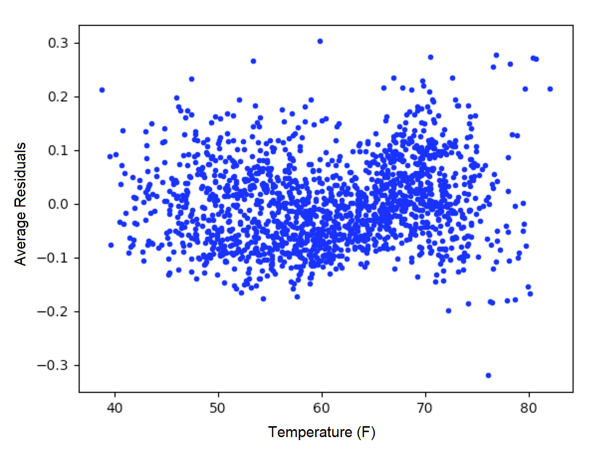
Figure: Average residuals vs. temperature
The average residuals vs. day-of-month graph did not show strong correlation between residuals and a particular day of the month.
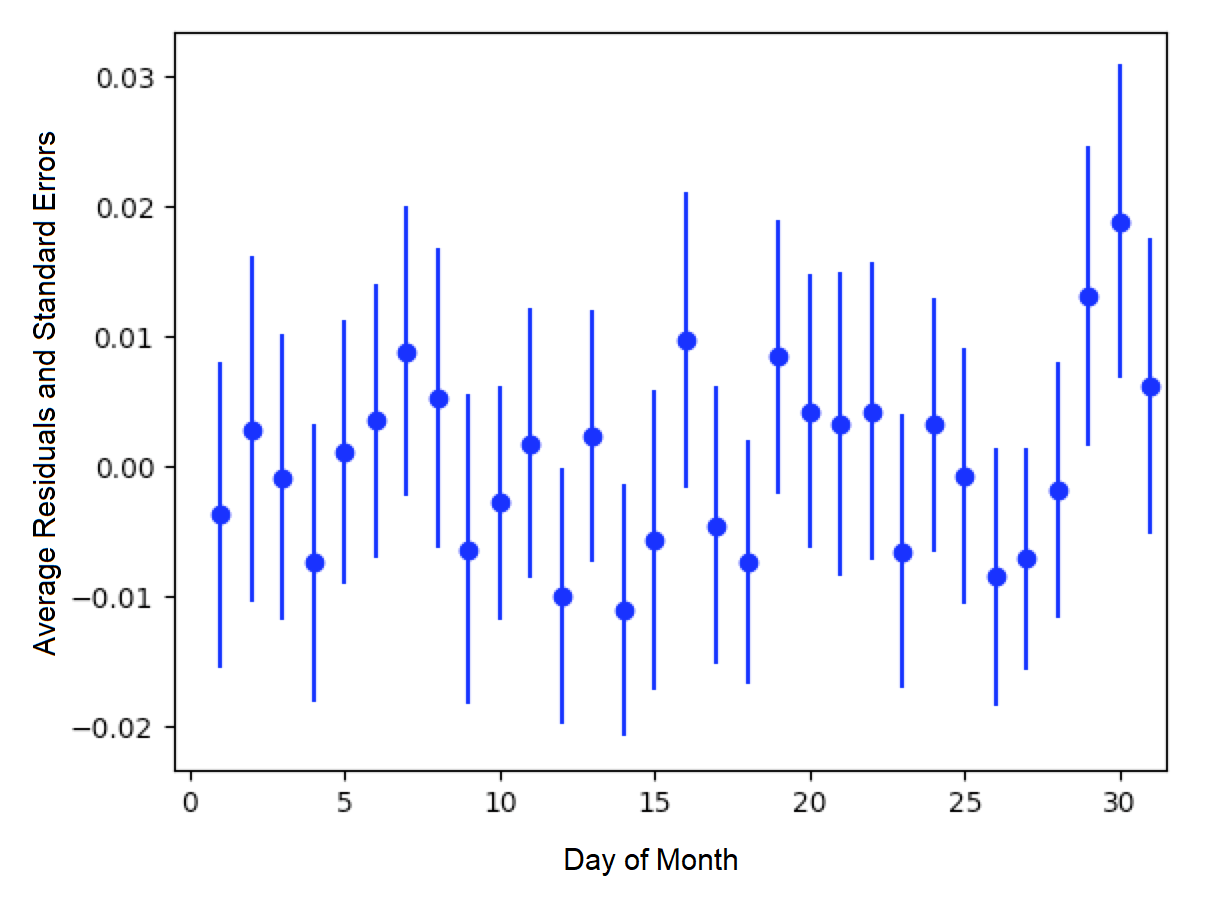
Figure: Average residuals vs. day-of-month
However, there did appear to be correlation between month-of-year and day-of-week with average residuals. The average residuals vs. month-of-year residuals graph shows positive and large residuals in the June, July, August, and December. The HDD and CDD covariates included in CalTRACK models control for temperature, which means this residual trend was not a first-order temperature effect. A possible explanation is that the high residual months coincided with months when school was not in session. School vacations likely result in higher household occupation and, thereby, higher energy consumption. This supports the inclusion of a month-of-day category variable.
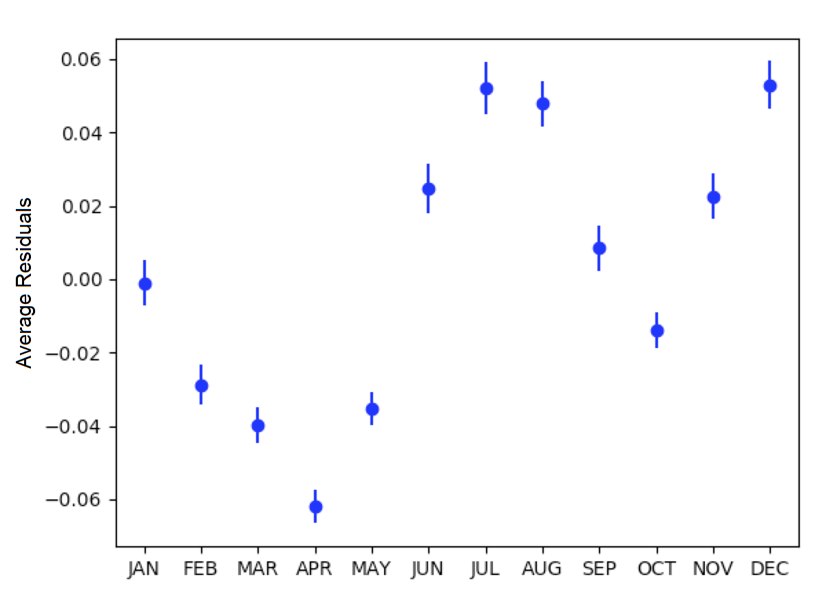
Figure: Average residuals vs. month-of-year
The average residuals vs. day-of-week graph shows a trend of large, positive residuals during the weekend days. It is reasonable to expect higher energy consumption during weekends because residents are more likely to be occupying the house. This supports the inclusion of a day-of-week category variable.
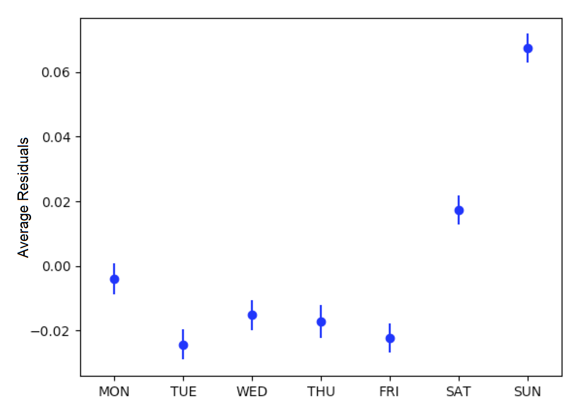
Figure: Average residuals vs. day-of-week
Finally, the average residuals were 0.061 for holidays and -0.001 for non-holidays. This indicates that energy consumption was higher during holidays than non-holidays for residential customers. This also supports the inclusion of a holiday indicator variable.
Test 2: Calendar effects and aggregated energy savings
Github issue: https://github.com/CalTRACK-2/caltrack/issues/57
Background:
Previous analysis showed temporal patterns in the residual structure for daily and billing period models, which suggests that calendar effects should be included in the billing period and daily CalTRACK model specifications. However, at the time of this testing, CalTRACK methods were designed to calculate only annual savings by aggregating building-level savings estimates over a year. For this reason, it is only necessary to include calendar effects in CalTRACK model specifications if they have a significant effect on annual savings calculations. The effect of adding calendar effects on annual energy savings was empirically tested as follows.
Tested parameters:
The empirical testing compared different model specifications with the following metrics:
- CVRMSE (Coefficient of Variation Root Mean Squared Error)
- NMBE (Normalized Mean Bias Error)
These are labels for the tested model specifications:
- M0: CalTRACK model with only HDD and CDD covariates
- M0.1: M0 but with a wide range of possible CDD/HDD balance points.
- M0.2: M0 but with robust regression and using the Huber loss function.
- M1: M0 plus a categorical day-of-week variable.
- M2: M0 plus a categorical variable distinguishing weekdays versus weekend days only.
- M3: M0 plus categorical day-of-week plus categorical month-of-year.
- M4: M1 with elastic net regularization (L1 = 0.5, L2 = 0.5).
- M5: M0.2 plus a categorical variable distinguishing weekdays versus weekend days only.
Testing methodology:
The testing methodology used out-of-sample data to estimate prediction error associated with each model specification of interest. Models with lower CVRMSE and a NMBE closer to 0 were preferred.
CalTRACK’s objectives prioritize simplicity in model specification decisions, so less complex model specifications were desired if they did not significantly detract from the quality of aggregated annual energy savings calculations.
Results:
The graph below presents the median CVRMSE and NMBE for each model specification. The results indicate that model M1 and M2, which included day-of-week and weekday or weekend indicator variables, respectively, generated only slightly lower CVRMSE and NMBE than the M0.1 model.
Additionally, it is clear that the two models with robust regression specifications generated much lower NMBE than the non-robust regression results. This is an important finding and a further discussion of robust regression is found in appendix 3.4.1.
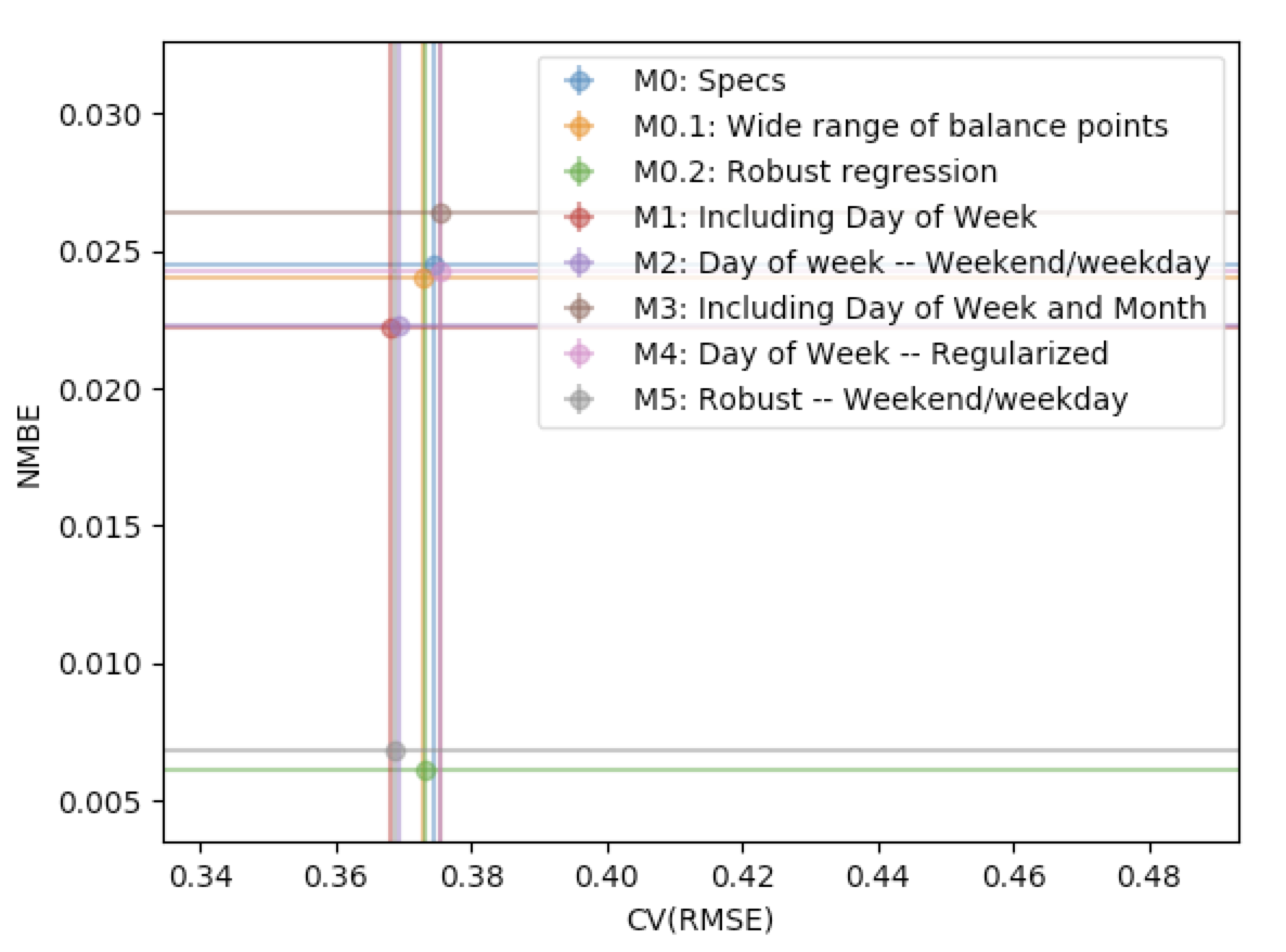
Figure: CVRMSE vs. NMBE
Conclusion:
Although adding calendar effects may be significant when estimating daily models, their effect is reduced when aggregated over a year. The small reductions in CVRMSE and NMBE gained by adding calendar effects do not justify their added complexity to CalTRACK models.
3.4.1. Models using daily data are fit using ordinary least squares.
Github issue: https://github.com/CalTRACK-2/caltrack/issues/57
Background:
In the context of home energy modelling, robust regressions tend to generate a normalized mean bias error (NMBE) that is closer to zero than ordinary least squares (OLS). This trend is apparent in the figure below, which presents the distribution of NMBE for robust regression and OLS with no calendar effects. The results show that OLS tended to predict higher energy usage, while robust regression tended to predict lower energy usage.
Robust regressions are computationally intensive and may be difficult to replicate across statistical software packages and CalTRACK methods value simplicity and replicability. This makes OLS preferable unless robust regression provides significantly better results than OLS.
Tested parameters:
The NMBE for CalTRACK models with robust regression and OLS were compared. Additionally, the computation requirements for robust regression and OLS were recorded and compared to further inform the decision.
Testing methodology:
Robust and OLS regressions were estimated and their NMBE was calculated. The computational requirements for each of these methods was also analyzed.
Results:
The empirical results below show that robust regression generates NMBE that are slightly closer to zero than OLS. The OLS models tend to have positive NMBE, while the robust regression has negative NMBE. Although the model fit was slightly better for robust regression, the robust regression took nearly 3 times longer to calculate than OLS. These were significant additional computation requirements for robust regression.
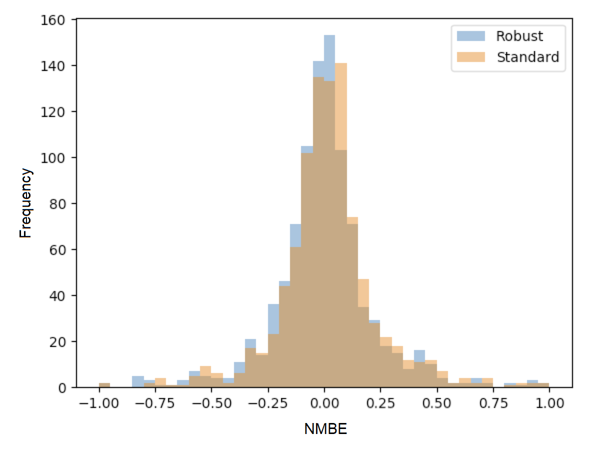
Figure: Distribution of NMBE for robust regression and ordinary least squares
Conclusion:
CalTRACK recommends using an OLS modelling approach instead of robust regression. The additional computation requirements and difficulties replicating robust regression across statistical packages are not justified by the small improvements to model fit from robust regression.
3.4.3.2. Candidate model qualification.
Github issue: https://github.com/CalTRACK-2/caltrack/issues/76
Background:
After HDD + CDD, HDD-only, CDD-only, and intercept-only model candidates are estimated, the best-fit model is selected through a two-stage process.
First, for each model specifications with covariates (HDD + CDD, HDD-only, and CDD-only), the estimated model’s HDD and CDD covariates that are statistically insignificant (p-value > .10) are removed from consideration. This is referred to as the p-value screen.
Second, the remaining model with the highest R-squared value is selected.
The p-value screen is conducted because statistically insignificant coefficients may lead to poor out-of-sample prediction. However, this procedure may eliminate best-fit candidate models. Additionally, models with estimates for HDD and CDD have more interpretation value than models with only HDD, CDD, or an intercept.
The effect of the p-value screen on out-of-sample error was analyzed to determine if the p-value screen improved model selection.
Data:
Billing period data from approximately 1000 residential buildings in Oregon.
Tested parameters:
The out-of-sample prediction errors were calculated for models selected with and without the p-value criterion.
Testing methodology:
- Caltrack monthly models were fit to the baseline period usage data using the p-value screen.
- The fitting process was repeated without a p-value screen.
- A comparison was performed using 24-month electric traces, split into 12 months of training and 12 months of test data. Mean absolute prediction error was used as the metric to compare performance.
Acceptance criteria:
This update was accepted if removing the p-value screen did not cause average model performance to deteriorate.
Results:
The graph below shows that the distribution of selected model types for the 1,000 building sample changed slightly when models were selected without a p-value screen. In almost 90% of the buildings, the fit did not change when the p-value criterion was removed. For the remainder that did change, the model shifted from an intercept-only model to a weather-sensitive model.
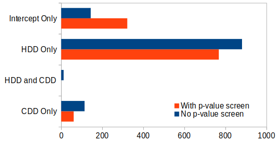
Figure: Best-fit model with p-value screen
The out-of-sample prediction for models selected with and without the p-value screen is graphed below. The average Mean Absolute Error (MAE) was 8.20 when the p-value screen was removed and 8.34 with the p-value screen. This indicates a slight improvement in prediction error when the p-value screen was eliminated. Additionally, over two times more models had improved model fit when the p-value screen was eliminated. Of the models that degraded when the p-value screen was eliminated, none of the degradations were catastrophic.
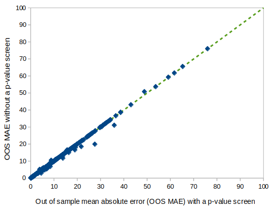
Figure: Mean absolute error with and without p-value screen
Conclusion:
Our tests indicate that requiring a P-value screen was superfluous at best and marginally counterproductive at worst. Therefore, the required P-value screen for candidate models will be removed from CalTRACK model selection criteria.
3.4.3.3. The model with highest adjusted R-squared will be selected as the final model.
Github issue: https://github.com/CalTRACK-2/caltrack/issues/62
Background:
CalTRACK grid search algorithm determines the optimal balance point temperatures by estimating a model for each HDD and CDD balance point in the grid search range and selecting the best-fit model. The definition of “best-fit” depends on the loss function. There are a variety of loss functions that are more or less suitable for different data structures and modelling methods.
The loss function candidates analyzed were:
- Quadratic Loss Function (referred to in the figure below as “least squares”)
- Linear Loss Function (referred to in the figure below as “absolute value”)
- Huber Loss Function
- Tukey’s Bi-square Loss Function
The distributions of each candidate loss function are visualized in the graph below. Of the candidate loss functions, the “Least Squares” or Quadratic Loss Function is the most common. It evaluates “best-fit” by selecting the model that minimizes the sum of squared residuals, which will also result in the highest R-Squared model. The Quadratic Loss Function is not robust to outliers.
The Tukey Bi-Square Loss Function is the most robust to outliers, but generates larger model variance in the absence of outliers.
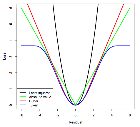
Figure: Loss function distributions
Empirical testing was conducted to determine the loss function that resulted in the best-fit balance point temperature models.
Tested parameters:
The HDD balance points were analyzed for each candidate loss function. They were evaluated based on the standard deviations of their estimated HDD balance points.
Testing methodology:
From the 1,000 residential building data set, the 263 buildings that were best fit by an CDD + HDD model were filtered for closer examination. Excluded models either had no significant heating or cooling component or were intercept-only models.
For each of the 263 selected buildings, the balance point algorithm was conducted 25 times. Before each test run, 10% of days in the baseline period were randomly removed. The selected balance point temperatures should not change drastically when 10% of days are removed from the baseline period. If the balance points do show large deviations between test runs, then it is possible that outliers are driving the fit.
The algorithm for selecting balance points operated as follows:
- Choose relevant balance points to test, which is determined by the grid search range and search increment
- Run a linear regression using the HDD and CDD values for each candidate balance point combination. Qualifying models must have non-negative intercept, heating, and cooling coefficients, and the heating and cooling coefficients must be statistically significant.
- Calculate the loss function.
- Choose new balance points and repeat.
- Select the balance points with the lowest loss function.
Our testing methodology used the balance point selection algorithm for each qualifying building 25 times with a different 10% of days removed from the baseline period. The mean and standard deviations for each home across the 25 test runs were calculated and recorded. This was repeated for each of the 4 candidate loss functions.
Results:
The frequency of selected balance points for each candidate loss function are shown in the graph below. It is apparent that the quadratic loss function was concentrated near the 65 F balance point. The high frequency of balance points at one temperature indicates that the quadratic loss function was not heavily skewed by outliers in this dataset.
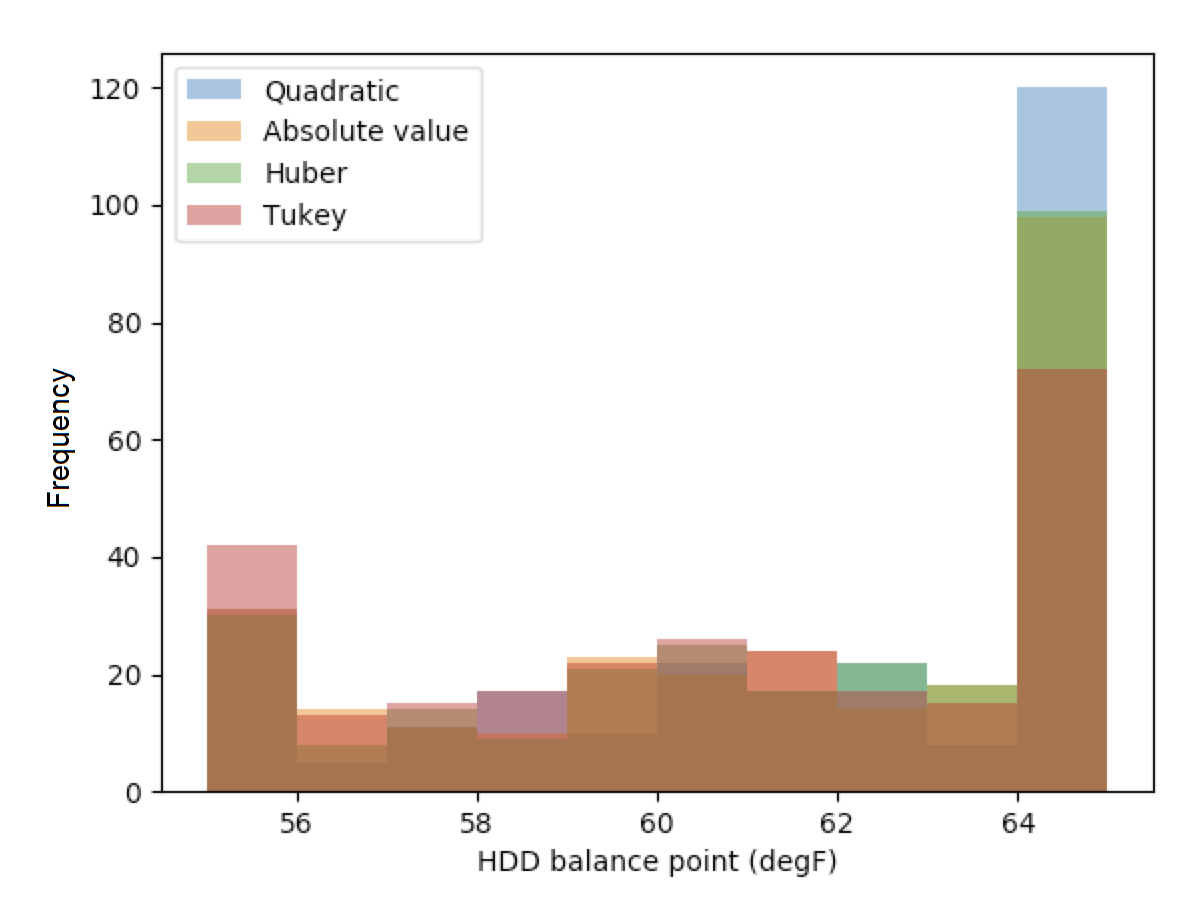
Figure: Frequency of balance point temperatures by loss function
These results are confirmed by analyzing standard deviations of balance points for each loss function. The empirical results below indicate that the quadratic loss function is the most stable among candidate loss functions.
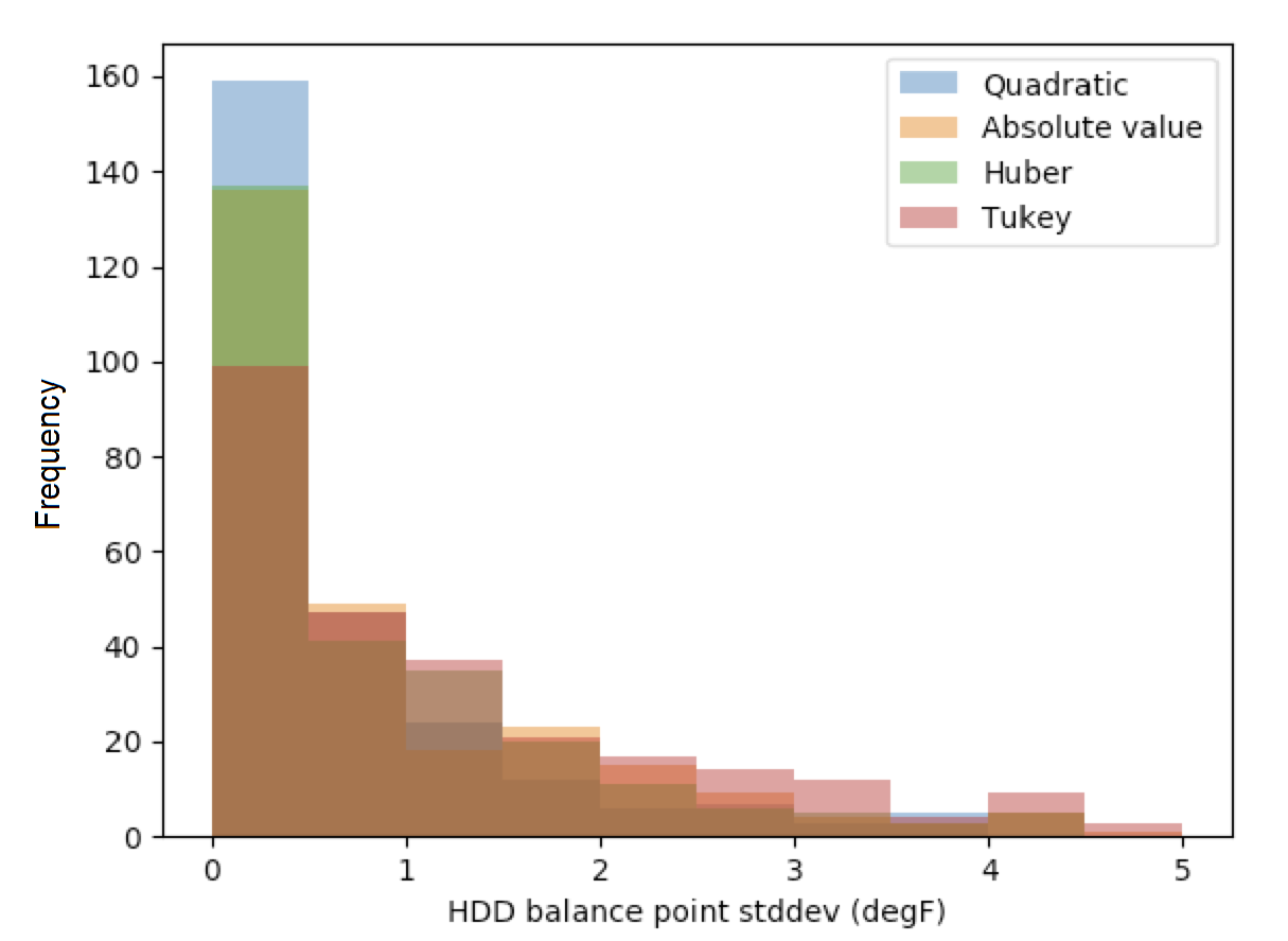
Figure: Balance point standard deviation by loss function
The “Frequency of balance point temperatures by loss function” bar chart shows that the quadratic loss function produced balance point temperatures concentrated at 65 F. It is possible that the grid search range was overly constrained, which caused HDD temperatures above 65 F to bunch on the edge of the grid search range.
The figure below presents the standard deviations of each candidate loss function with balance point temperatures at either 55 F or 65 F removed from the sample. This eliminated HDD balance points that were bunched at either edge of the grid search range. The results still showed that the quadratic loss function generated balance points with the smallest standard deviations.
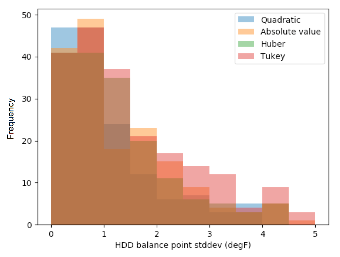
Figure: Balance point standard deviation by loss function (edges removed)
The quadratic loss function performed the best among candidate loss functions. The bar chart below shows the standard deviation of balance point temperatures across test runs evaluated with the quadratic loss function. These results indicate that 80% of the sample has balance point temperature standard deviations of less than 1 degree.
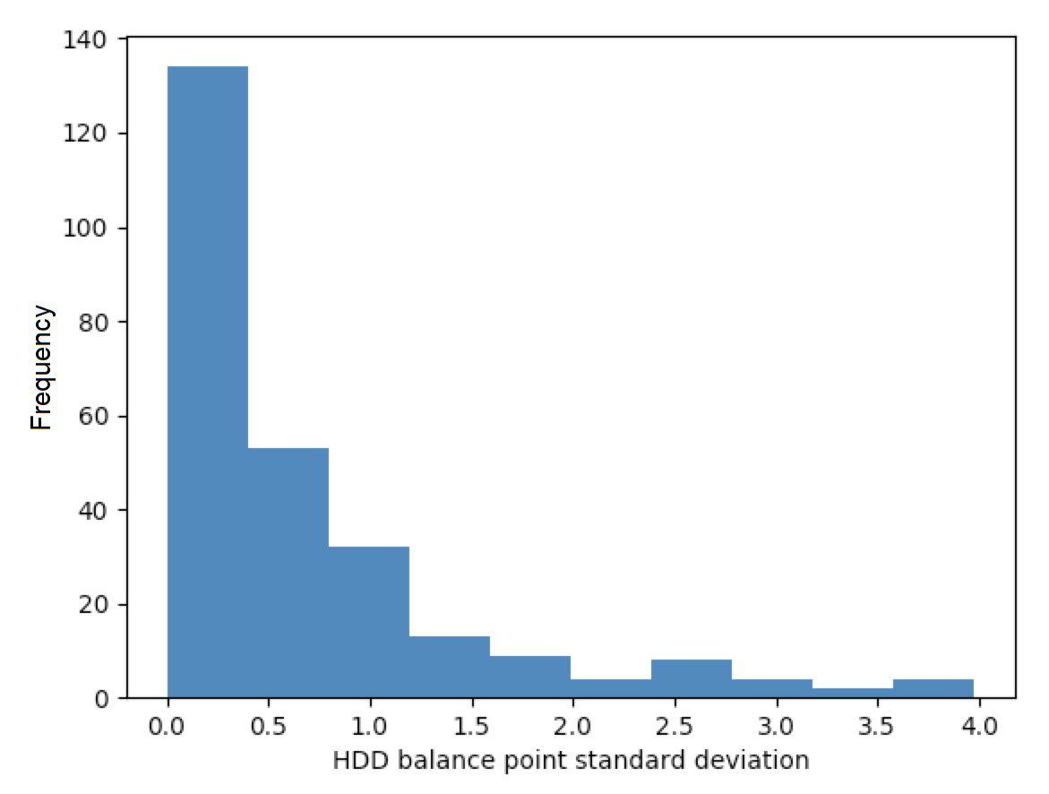
Figure: Quadratic loss function balance point standard deviations
Conclusion:
Our results indicate that the quadratic loss function produced the most stable results across the test data set. Under the quadratic loss function, 80% of buildings had standard deviations of 1 F or less. This is the recommended loss function for CalTRACK methods.
3.6.5. Baseline periods.
Test 1: Adequacy of single estimated regression for baseline period
Github issue: https://github.com/CalTRACK-2/caltrack/issues/103
Background:
The Time-Of-Week and Temperature model for hourly methods uses a single model to fit the entire baseline period, which could be up to 12 months long. The single, yearly regression approach assumes that baseline and weather-sensitive energy consumption is constant throughout the year.
However, it is possible that baseline and weather-sensitive energy consumption is not constant across the entire baseline period. For example, the baseline energy consumption may be higher during summer months than spring months because children do not spend daytime hours at school during the summer. If this is the case, then estimated parameters for a single, yearly regression will not reflect the true energy consumption during each month of the baseline period. This results in higher uncertainty of CalTRACK energy savings estimates.
Data:
Residential, daily electricity data from 80 buildings. Data was supplied by Home Energy Analytics.
Tested parameters:
The average CVRMSE from sampled buildings with different modelling approaches.
Testing methodology:
Energy savings for the 80 sampled households were calculated and compared when:
- A single, yearly regression was estimated for the entire baseline period
- 12 separate regressions were estimated for each month of the baseline period
The methods were evaluated based on the average CVRMSE of sampled households.
Results:
The results shows that CVRMSE was improved when regressions were estimated for each month of the baseline period. There were CVRMSE improvements of 33% and 19% for electric and gas respectively when regressions were estimated for each month of the baseline period.
The figure below shows a distinct difference between monthly and annual regressions. The baseline region, which is the green portion of the graphs, in the annual regression was constant across the entire year. However, when regressions are estimated for each month in the baseline period, it is clear that baseline energy consumption varied in different months of the year.
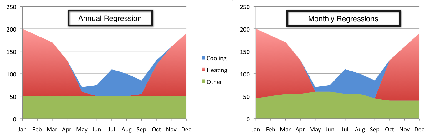
Figure: Annual vs. monthly regressions
Test 2: Optimal number of regressions in baseline period
Github issue: https://github.com/CalTRACK-2/caltrack/issues/85
Background:
In the context of hourly methods, it was established that a single estimated regression for the entire baseline period likely increases CVRMSE. One possible strategy to address this problem is estimating a regression for each month of the baseline period, which results in 12 estimated regressions. Unfortunately, models fit from limited time periods without enough data points may become overfit.
To determine the optimal number of regressions in the baseline period, the following regression intervals were tested and compared based on their in-sample and out-of-sample CVRMSE. The out-of-sample CVRMSE indicates if the model is overfit.
Regression intervals:
- Year-long baseline: One regression was estimated for the entire baseline period.
- 3-month baseline: A regression was estimated every 3 months of the baseline period.
- 3-month weighted baseline: A regression was estimated for each month of the baseline period, but the months before and after were included and weighted down by 50%.
- 3-month weighted baseline with holiday flags: This was the same as the 3-month weighted baseline but indicator variables for holidays were included in the regression specification.
- 1-month baseline: A regression was estimated for each month of the baseline period.
Data:
Hourly data from residential buildings in California.
Tested parameters:
The in-sample and out-of-sample CVRMSE were calculated for different numbers of regressions estimated in baseline period.
Testing methodology:
Models with the five candidate regression intervals were estimated and the CVRMSE for each of these was calculated with in-sample and out-of-sample data.
Results:
The graph below presents the in-sample and out-of-sample CVRMSE for each regression interval candidate. The optimal regression interval had the lowest in-sample CVRMSE without overfitting the model. The out-of-sample CVRMSE increases when the model was overfit.
The results show that the in-sample CVRMSE with a year-long baseline was much larger than the other regression intervals. The 1-month interval had the lowest in-sample CVRMSE, but had a larger out-of-sample CVRMSE than the 3-month and weighted 3-month baselines. This signals that the 1-month interval may overfit limited data.
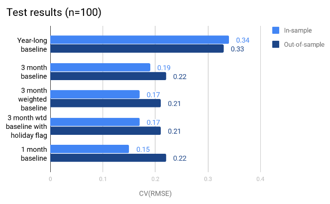
Figure: In- and out-of-sample CVRMSE
Conclusion:
The results showed that estimating a single regression for the entire baseline period likely increased the CVRMSE, which is not ideal for CalTRACK methods.
The 3-month weighted baseline is the preferred number of regressions for the baseline period. This approach accounts for variation in baseline energy consumption across months without overfitting the model to limited data.